A good way to determine if you have inserted the values correctly is to see if there are different colors in the chart. How to add error bars in Google Sheets?
Post navigation
If the issue is with your Computer or a Laptop you should try using Reimage Plus which can scan the repositories and replace corrupt and missing files. This works in most cases, where the issue is originated due to a system corruption. You can download Reimage by clicking the Download button below. Download Now. Now we want to fit a line to this scatterplot that best represents the relationship between the data.
Appendix G: Using Excel to Create a Graph with Error Bars
It looks like higher unemployment rates correspond to higher voting rates. To see what a linear relationship looks like, we fit a line to this figure. In the "Chart Layout" section at the top, there's an option called "Trendline. Selecting the " Linear Trendline " option will produce the following result supporting our assumption that higher unemployment rates correspond to higher voting rates:.
Fitting trendlines allows for many options. Sometimes, we can hypothesize that the relationship between our variables is not simply linear. For example, we hypothesize that the relationship of voting behavior over time is not linear.
- Post navigation;
- charts - how to add standard deviation error bars on excel - Super User?
- Subscribe to RSS.
- How to add error bars in Excel: standard and custom.
- Was this information helpful?;
- apple mac pro md878j a.
In the following case, we chose to plot an polynomial trendline and we can see that it bends downwards and then upwards as time increases. This relationship would not be visible if we used a linear trendline.
- mac os x mavericks wiki.
- Re: Range bars, not error bars;
- ctrl left click on mac.
- create new account mac os.
- How to add error bars in Excel: A quick tutorial ▷ newsroom.futurocoin.com?
- fifa 12 game free download for mac.
- ERC Tweets;
- Office 2011 for Mac All-in-One For Dummies;
- How to add error bars in Google Sheets? - newsroom.futurocoin.com?
- maquiagem com o batom diva da mac.
- chocolatier 2 secret ingredients mac.
You can edit your trendline and see more options by right-clicking on the chart field to select it and choosing "Format Trendline" from the menu. Apart from editing the visual appearance of our line, we can choose a number of other options. One of the most important is to display a measure of how well your linear relationship fits your data.
The R-squared value is a summary of how much of the variance a particular line explains. In the format box, check the boxes to display the equation and the R-squared values on your graph. We can now see the equation of the line and the proportion of variance in the data explained by the linear relationship. Visually, this is the same process as running a regression of the Y-variable on the X-variable.
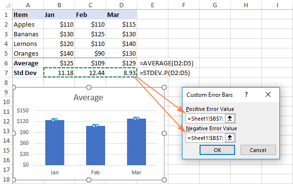
How To Create Custom Error Bars In Excel
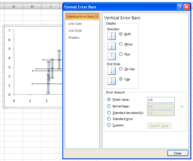
Here you set the display of the selected set of error bars. The formatting options for the selected category then appear in collapsible and expandable lists at the bottom of the task pane.
You can click the titles of each category list to expand and collapse the display of the options within that category. You can set any options that you would like within the task pane to immediately apply those changes to the chart. Try the Excel Course for Free!