Freeze or lock rows and columns in an Excel worksheet
Search form Search. Freeze or lock rows and columns in an Excel worksheet. Microsoft Excel. Why you might need to freeze rows or columns in your spreadsheet Imagine you have a spreadsheet that contains sales data for January. The worksheet contains daily data that reports the sales for each person in your sales team, broken down by products sold: This example actually has 85 rows of data the table carries on down further than this screenshot shows: Once you scroll down, however, the heading row disappears off the top of the screen, and you can no longer be sure what each column contains: This is a simple example, but it's not hard to imagine that with a lot more columns and rows, the problem would get considerably more complex, To solve the problem, you can freeze or lock the heading rows so that they don't disappear off the top of the screen as you scroll down the worksheet.
The proces for doing this is slightly different between Excel for Windows and Excel for Mac, so I've covered both here: How to freeze rows and columns You have two options for freezing panes in Excel.
Freeze panes to lock the first row or column
Note that these steps also apply to freezing columns: If you wanted to freeze the first column, you would then go back and choose that option. The screenshot below is from Excel for Windows. In the Mac version of Excel the options are the same, but you don't get the explanations of each option that you see here: Things get slightly more complicated if you want to freeze more than one row or column. If you look at the first screenshot in this lesson, you'll see that the first row doesn't actually contain the headings for the sales data table - it contains the title of this worksheet.
To freeze the heading row of the table, you will have to freeze the first five rows in the worksheet. To do this, click in the cell A6 i. When you do this, not much will appear to change.
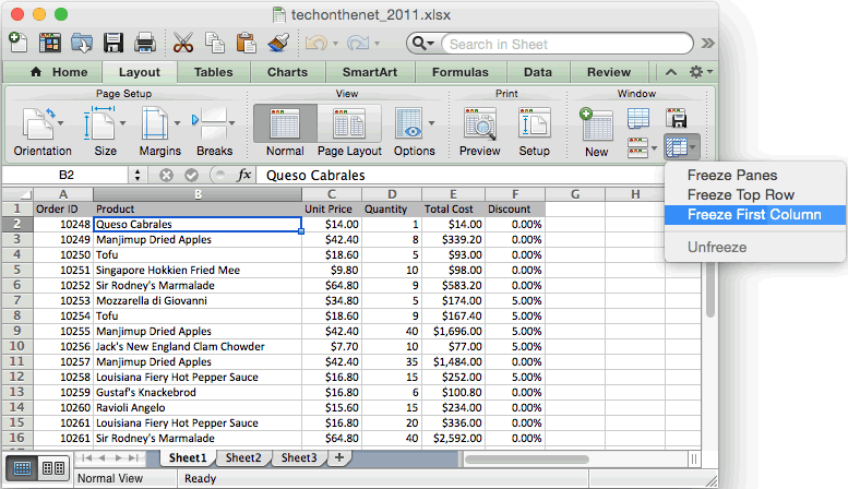
MS Excel for Mac: Freeze top row
All you'll see is a line stretching across the screen, almost like a border along the bottom of row 5 which is the last row to be frozen in our example. The screenshot shows what Freeze Panes looks like if you had clicked B6 before clicking Freeze Panes i.
Here's what the sales data table looks like if you scroll down. As you can see, the first five rows have stayed put, and the other rows have disappeared underneath them as I've scrolled down the screen: How to unfreeze panes in Excel Unfreezing panes is, fortunately, fairly simple: The first option, which was Freeze Panes, is now Unfreeze Panes. Click that option and the frozen rows will be unfrozen. In Excel for Mac, choose the Layout menu and choose Unfreeze Panes for some reason, it's a separate option which only becomes available once you have frozen panes.
Want to learn more? Try these lessons: Scale your Excel spreadsheet to fit your screen. Print header rows at the top of every page in Excel for Mac. Tell us about your experience with our site.
PGB1 Created on December 19, Good Morning! I tried other options in the drop-down too. I've also tried clicking different cells in the row below the rows I wish to freeze.
- mac kohl eyeliner pencil review.
- how to install windows games on mac os.
- fraps free full version download mac.
So, do you all know where I'm goofing up? This thread is locked. You can follow the question or vote as helpful, but you cannot reply to this thread. I have the same question Want to unfreeze a row, column, or both?
On the View tab, click Unfreeze Panes. Expand your Office skills. Get new features first. Was this information helpful?
Yes No. Any other feedback? How can we improve it? Send No thanks.