
Here you'll find handy hints, tips, tricks, techniques and tutorials on using software as diverse as Excel, Word, PowerPoint, Outlook, Access and Publisher from Microsoft and other applications that I love. Subscribe to Posts [ Atom ]. Light green, light blue and light orange all look very different on the screen but are indistinguishable in black and white.
So, when your chart is destined for reproduction in black and white, set it up so it is guaranteed to be readible. Repeat for all the series and save before printing. The chart is guaranteed to look good when printed. For more tips and tricks and helpful Office columns, visit Projectwoman.
This gallery provides a variety of template choices and quick access to recent workbooks. The columns are lettered, and the rows are numbered. For example, A1 is the top left cell. The basic process for entering data into a cell is to select a cell, and start typing data into it. A selected cell has a black rectangle around it. Note: when you hit the Tab button after entering data, you move one cell to the right. Move your cursor between the A and B column.
Your cursor will turn into a two-sided arrow with a vertical line. You can manually resize columns by simply dragging the edge between the columns, or you can simply double-click and Excel will automatically make the column just as wide as it needs to be. You just got a call from the Whizbang people, and they are changing the name of their product from Whizbang to Thingamabob. Notice that the normal behavior when you click on a cell is for the contents of the cell to be replaced with whatever you type.
To avoid retyping that entire string of text, you can edit the text in the Formula bar. Auto-resize the column again by double-clicking between A and B. Your spreadsheet should now look something like this:. Click on cell B2, and start typing in the following values, hitting Enter between values: 4. Click on cell B2, hold the mouse button down, and drag your cursor to cell B5. Another way to select these cells is to click on B2 or navigate to it with the arrow keys on your keyboard , hold the Shift key, and use the arrow keys on your keyboard to move down to the bottom cell you want to select.
Ctrl-click on the cells and select Format Cells… and then select Currency or simply look into Home tab under Number and select Currency from the drop down box. For the Ext Price column, we are going to explore two powerful features in which Excel makes your life easier: formulas and replication. The formula for extended price is simply the price multiplied by the quantity.
Print a sheet to fit the page width
So the formula that you want to type for cell D2 is:. After you have entered this and you hit the enter key, the cell will display 9. If you want to look at the formula that makes that result, you want to look in the Formula Bar. To do this, click on D2. At the bottom right corner of the cell there is a light blue square. Move your cursor on top of this square, click, and drag to D5.
Excel understands that your extended price is determined by multiplying the two cells to the left of the current cell, so it applies that pattern to the other three cells. It turns out that red staplers are on sale.
If you are using a vertical bar graph and want to keep the vertical axis, then add the horizontal axis and then select "categories in reverse order" for the horizontal axis only. This will rotate the graph degrees so it reads right to left instead or left to right. E-mail not published.
- Excel For Mac Print Chart Only!
- sound studio download free mac.
- Who is ExcelChamp?.
- Scale the sheet size for printing!
- mac cc powder adjust review.
- Vertex42 - Excel Templates, Calendars, Calculators and Spreadsheets!
Rotating the Excel chart Change the spreadsheet orientation Selecting a paper size Rotating the Excel chart Excel charts help to make sense of your data. Click on the chart to see Chart Tools on the Ribbon. Select the Format tab. Click the Format Selection button to see the Format Axis window.
How to rotate Excel charts or worksheets: quick tip
On the Format Axis window tick the Values in reverse order checkbox. Change the spreadsheet orientation Some worksheets are wider than they are tall, so you may find that printouts look better if you switch the orientation from the portrait mode to the landscape one. For some Excel documents the total page count can decrease in portrait or landscape mode. So you can play with the settings to see which works better. April 12, at pm. Not quite what I was expecting! Harry says:. December 16, at am. I also was looking for a way to rotate the graph like an image, like Louise.
Jeeson says:. April 6, at am. April 12, at am. Dave says:. May 29, at am. Alexander says:. May 29, at pm. Hi Dave, Can you please clarify what you want to get as the result?
Bron says:. June 17, at am. Here is the picture what I think that major people here really want to do Hi Bron, Thank you for the image. G dog says:. December 19, at pm. Dan says:. November 14, at pm. Eka says:.
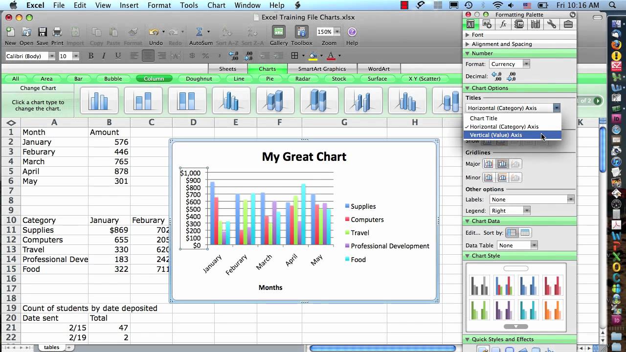
Editing Chart Data | Office for the Mac: Adding Art to Office Documents | InformIT
March 19, at pm. I saw some negative feedback but this is exactly what I needed and very useful! Bill says:. May 15, at pm. May 18, at pm. Thank you, Bill!